House Prices Advanced Regression Techniques V2
Kaggle Competition 的练习
# 安装 vecstack
!pip install vecstack
# 数据分析库
import pandas as pd
import numpy as np
import random

# 数据可视化
import seaborn as sns
import matplotlib.pyplot as plt
plt.style.use('ggplot')

# 机器学习库
from sklearn.preprocessing import OneHotEncoder
from sklearn.linear_model import LogisticRegression
from sklearn.svm import SVC, LinearSVC
from sklearn.ensemble import RandomForestRegressor, AdaBoostRegressor, GradientBoostingRegressor, BaggingRegressor
from sklearn.neighbors import KNeighborsClassifier
from sklearn.naive_bayes import GaussianNB
from sklearn.linear_model import Perceptron
from sklearn.linear_model import SGDClassifier
from sklearn.tree import DecisionTreeClassifier
from sklearn.metrics import r2_score, mean_squared_error
from sklearn.model_selection import RandomizedSearchCV, cross_val_score, StratifiedKFold, learning_curve, KFold, train_test_split

# Ensemble Models
from xgboost import XGBRegressor
from lightgbm import LGBMRegressor

# Package for stacking models
from vecstack import stacking
导入数据
train = pd.read_csv('/train.csv', index_col='Id')
test = pd.read_csv('/test.csv', index_col='Id')

train.head()
| MSSubClass | MSZoning | LotFrontage | LotArea | Street | Alley | LotShape | LandContour | Utilities | LotConfig | LandSlope | Neighborhood | Condition1 | Condition2 | BldgType | HouseStyle | OverallQual | OverallCond | YearBuilt | YearRemodAdd | RoofStyle | RoofMatl | Exterior1st | Exterior2nd | MasVnrType | MasVnrArea | ExterQual | ExterCond | Foundation | BsmtQual | BsmtCond | BsmtExposure | BsmtFinType1 | BsmtFinSF1 | BsmtFinType2 | BsmtFinSF2 | BsmtUnfSF | TotalBsmtSF | Heating | HeatingQC | CentralAir | Electrical | 1stFlrSF | 2ndFlrSF | LowQualFinSF | GrLivArea | BsmtFullBath | BsmtHalfBath | FullBath | HalfBath | BedroomAbvGr | KitchenAbvGr | KitchenQual | TotRmsAbvGrd | Functional | Fireplaces | FireplaceQu | GarageType | GarageYrBlt | GarageFinish | GarageCars | GarageArea | GarageQual | GarageCond | PavedDrive | WoodDeckSF | OpenPorchSF | EnclosedPorch | 3SsnPorch | ScreenPorch | PoolArea | PoolQC | Fence | MiscFeature | MiscVal | MoSold | YrSold | SaleType | SaleCondition | SalePrice | |
|---|---|---|---|---|---|---|---|---|---|---|---|---|---|---|---|---|---|---|---|---|---|---|---|---|---|---|---|---|---|---|---|---|---|---|---|---|---|---|---|---|---|---|---|---|---|---|---|---|---|---|---|---|---|---|---|---|---|---|---|---|---|---|---|---|---|---|---|---|---|---|---|---|---|---|---|---|---|---|---|---|
| Id | ||||||||||||||||||||||||||||||||||||||||||||||||||||||||||||||||||||||||||||||||
| 1 | 60 | RL | 65.0 | 8450 | Pave | NaN | Reg | Lvl | AllPub | Inside | Gtl | CollgCr | Norm | Norm | 1Fam | 2Story | 7 | 5 | 2003 | 2003 | Gable | CompShg | VinylSd | VinylSd | BrkFace | 196.0 | Gd | TA | PConc | Gd | TA | No | GLQ | 706 | Unf | 0 | 150 | 856 | GasA | Ex | Y | SBrkr | 856 | 854 | 0 | 1710 | 1 | 0 | 2 | 1 | 3 | 1 | Gd | 8 | Typ | 0 | NaN | Attchd | 2003.0 | RFn | 2 | 548 | TA | TA | Y | 0 | 61 | 0 | 0 | 0 | 0 | NaN | NaN | NaN | 0 | 2 | 2008 | WD | Normal | 208500 |
| 2 | 20 | RL | 80.0 | 9600 | Pave | NaN | Reg | Lvl | AllPub | FR2 | Gtl | Veenker | Feedr | Norm | 1Fam | 1Story | 6 | 8 | 1976 | 1976 | Gable | CompShg | MetalSd | MetalSd | None | 0.0 | TA | TA | CBlock | Gd | TA | Gd | ALQ | 978 | Unf | 0 | 284 | 1262 | GasA | Ex | Y | SBrkr | 1262 | 0 | 0 | 1262 | 0 | 1 | 2 | 0 | 3 | 1 | TA | 6 | Typ | 1 | TA | Attchd | 1976.0 | RFn | 2 | 460 | TA | TA | Y | 298 | 0 | 0 | 0 | 0 | 0 | NaN | NaN | NaN | 0 | 5 | 2007 | WD | Normal | 181500 |
| 3 | 60 | RL | 68.0 | 11250 | Pave | NaN | IR1 | Lvl | AllPub | Inside | Gtl | CollgCr | Norm | Norm | 1Fam | 2Story | 7 | 5 | 2001 | 2002 | Gable | CompShg | VinylSd | VinylSd | BrkFace | 162.0 | Gd | TA | PConc | Gd | TA | Mn | GLQ | 486 | Unf | 0 | 434 | 920 | GasA | Ex | Y | SBrkr | 920 | 866 | 0 | 1786 | 1 | 0 | 2 | 1 | 3 | 1 | Gd | 6 | Typ | 1 | TA | Attchd | 2001.0 | RFn | 2 | 608 | TA | TA | Y | 0 | 42 | 0 | 0 | 0 | 0 | NaN | NaN | NaN | 0 | 9 | 2008 | WD | Normal | 223500 |
| 4 | 70 | RL | 60.0 | 9550 | Pave | NaN | IR1 | Lvl | AllPub | Corner | Gtl | Crawfor | Norm | Norm | 1Fam | 2Story | 7 | 5 | 1915 | 1970 | Gable | CompShg | Wd Sdng | Wd Shng | None | 0.0 | TA | TA | BrkTil | TA | Gd | No | ALQ | 216 | Unf | 0 | 540 | 756 | GasA | Gd | Y | SBrkr | 961 | 756 | 0 | 1717 | 1 | 0 | 1 | 0 | 3 | 1 | Gd | 7 | Typ | 1 | Gd | Detchd | 1998.0 | Unf | 3 | 642 | TA | TA | Y | 0 | 35 | 272 | 0 | 0 | 0 | NaN | NaN | NaN | 0 | 2 | 2006 | WD | Abnorml | 140000 |
| 5 | 60 | RL | 84.0 | 14260 | Pave | NaN | IR1 | Lvl | AllPub | FR2 | Gtl | NoRidge | Norm | Norm | 1Fam | 2Story | 8 | 5 | 2000 | 2000 | Gable | CompShg | VinylSd | VinylSd | BrkFace | 350.0 | Gd | TA | PConc | Gd | TA | Av | GLQ | 655 | Unf | 0 | 490 | 1145 | GasA | Ex | Y | SBrkr | 1145 | 1053 | 0 | 2198 | 1 | 0 | 2 | 1 | 4 | 1 | Gd | 9 | Typ | 1 | TA | Attchd | 2000.0 | RFn | 3 | 836 | TA | TA | Y | 192 | 84 | 0 | 0 | 0 | 0 | NaN | NaN | NaN | 0 | 12 | 2008 | WD | Normal | 250000 |
浏览数据
train.info()
<class 'pandas.core.frame.DataFrame'>
Int64Index: 1460 entries, 1 to 1460
Data columns (total 80 columns):
MSSubClass 1460 non-null int64
MSZoning 1460 non-null object
LotFrontage 1201 non-null float64
LotArea 1460 non-null int64
Street 1460 non-null object
Alley 91 non-null object
LotShape 1460 non-null object
LandContour 1460 non-null object
Utilities 1460 non-null object
LotConfig 1460 non-null object
LandSlope 1460 non-null object
Neighborhood 1460 non-null object
Condition1 1460 non-null object
Condition2 1460 non-null object
BldgType 1460 non-null object
HouseStyle 1460 non-null object
OverallQual 1460 non-null int64
OverallCond 1460 non-null int64
YearBuilt 1460 non-null int64
YearRemodAdd 1460 non-null int64
RoofStyle 1460 non-null object
RoofMatl 1460 non-null object
Exterior1st 1460 non-null object
Exterior2nd 1460 non-null object
MasVnrType 1452 non-null object
MasVnrArea 1452 non-null float64
ExterQual 1460 non-null object
ExterCond 1460 non-null object
Foundation 1460 non-null object
BsmtQual 1423 non-null object
BsmtCond 1423 non-null object
BsmtExposure 1422 non-null object
BsmtFinType1 1423 non-null object
BsmtFinSF1 1460 non-null int64
BsmtFinType2 1422 non-null object
BsmtFinSF2 1460 non-null int64
BsmtUnfSF 1460 non-null int64
TotalBsmtSF 1460 non-null int64
Heating 1460 non-null object
HeatingQC 1460 non-null object
CentralAir 1460 non-null object
Electrical 1459 non-null object
1stFlrSF 1460 non-null int64
2ndFlrSF 1460 non-null int64
LowQualFinSF 1460 non-null int64
GrLivArea 1460 non-null int64
BsmtFullBath 1460 non-null int64
BsmtHalfBath 1460 non-null int64
FullBath 1460 non-null int64
HalfBath 1460 non-null int64
BedroomAbvGr 1460 non-null int64
KitchenAbvGr 1460 non-null int64
KitchenQual 1460 non-null object
TotRmsAbvGrd 1460 non-null int64
Functional 1460 non-null object
Fireplaces 1460 non-null int64
FireplaceQu 770 non-null object
GarageType 1379 non-null object
GarageYrBlt 1379 non-null float64
GarageFinish 1379 non-null object
GarageCars 1460 non-null int64
GarageArea 1460 non-null int64
GarageQual 1379 non-null object
GarageCond 1379 non-null object
PavedDrive 1460 non-null object
WoodDeckSF 1460 non-null int64
OpenPorchSF 1460 non-null int64
EnclosedPorch 1460 non-null int64
3SsnPorch 1460 non-null int64
ScreenPorch 1460 non-null int64
PoolArea 1460 non-null int64
PoolQC 7 non-null object
Fence 281 non-null object
MiscFeature 54 non-null object
MiscVal 1460 non-null int64
MoSold 1460 non-null int64
YrSold 1460 non-null int64
SaleType 1460 non-null object
SaleCondition 1460 non-null object
SalePrice 1460 non-null int64
dtypes: float64(3), int64(34), object(43)
memory usage: 923.9+ KB
train.describe(include="O")
| MSZoning | Street | Alley | LotShape | LandContour | Utilities | LotConfig | LandSlope | Neighborhood | Condition1 | Condition2 | BldgType | HouseStyle | RoofStyle | RoofMatl | Exterior1st | Exterior2nd | MasVnrType | ExterQual | ExterCond | Foundation | BsmtQual | BsmtCond | BsmtExposure | BsmtFinType1 | BsmtFinType2 | Heating | HeatingQC | CentralAir | Electrical | KitchenQual | Functional | FireplaceQu | GarageType | GarageFinish | GarageQual | GarageCond | PavedDrive | PoolQC | Fence | MiscFeature | SaleType | SaleCondition | |
|---|---|---|---|---|---|---|---|---|---|---|---|---|---|---|---|---|---|---|---|---|---|---|---|---|---|---|---|---|---|---|---|---|---|---|---|---|---|---|---|---|---|---|---|
| count | 1460 | 1460 | 91 | 1460 | 1460 | 1460 | 1460 | 1460 | 1460 | 1460 | 1460 | 1460 | 1460 | 1460 | 1460 | 1460 | 1460 | 1452 | 1460 | 1460 | 1460 | 1423 | 1423 | 1422 | 1423 | 1422 | 1460 | 1460 | 1460 | 1459 | 1460 | 1460 | 770 | 1379 | 1379 | 1379 | 1379 | 1460 | 7 | 281 | 54 | 1460 | 1460 |
| unique | 5 | 2 | 2 | 4 | 4 | 2 | 5 | 3 | 25 | 9 | 8 | 5 | 8 | 6 | 8 | 15 | 16 | 4 | 4 | 5 | 6 | 4 | 4 | 4 | 6 | 6 | 6 | 5 | 2 | 5 | 4 | 7 | 5 | 6 | 3 | 5 | 5 | 3 | 3 | 4 | 4 | 9 | 6 |
| top | RL | Pave | Grvl | Reg | Lvl | AllPub | Inside | Gtl | NAmes | Norm | Norm | 1Fam | 1Story | Gable | CompShg | VinylSd | VinylSd | None | TA | TA | PConc | TA | TA | No | Unf | Unf | GasA | Ex | Y | SBrkr | TA | Typ | Gd | Attchd | Unf | TA | TA | Y | Gd | MnPrv | Shed | WD | Normal |
| freq | 1151 | 1454 | 50 | 925 | 1311 | 1459 | 1052 | 1382 | 225 | 1260 | 1445 | 1220 | 726 | 1141 | 1434 | 515 | 504 | 864 | 906 | 1282 | 647 | 649 | 1311 | 953 | 430 | 1256 | 1428 | 741 | 1365 | 1334 | 735 | 1360 | 380 | 870 | 605 | 1311 | 1326 | 1340 | 3 | 157 | 49 | 1267 | 1198 |
检查缺失数据
train_missing = train.isnull().sum()
train_missing = train_missing[train_missing > 0]
train_missing
LotFrontage 259
Alley 1369
MasVnrType 8
MasVnrArea 8
BsmtQual 37
BsmtCond 37
BsmtExposure 38
BsmtFinType1 37
BsmtFinType2 38
Electrical 1
FireplaceQu 690
GarageType 81
GarageYrBlt 81
GarageFinish 81
GarageQual 81
GarageCond 81
PoolQC 1453
Fence 1179
MiscFeature 1406
dtype: int64
test_missing = test.isnull().sum()
test_missing = test_missing[test_missing > 0]
test_missing
MSZoning 4
LotFrontage 227
Alley 1352
Utilities 2
Exterior1st 1
Exterior2nd 1
MasVnrType 16
MasVnrArea 15
BsmtQual 44
BsmtCond 45
BsmtExposure 44
BsmtFinType1 42
BsmtFinSF1 1
BsmtFinType2 42
BsmtFinSF2 1
BsmtUnfSF 1
TotalBsmtSF 1
BsmtFullBath 2
BsmtHalfBath 2
KitchenQual 1
Functional 2
FireplaceQu 730
GarageType 76
GarageYrBlt 78
GarageFinish 78
GarageCars 1
GarageArea 1
GarageQual 78
GarageCond 78
PoolQC 1456
Fence 1169
MiscFeature 1408
SaleType 1
dtype: int64
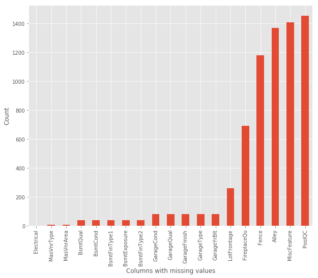
# 可视化缺失数据
def plot_missing(df):
# 寻找缺失的列
missing = df.isnull().sum()
missing = missing[missing > 0]
missing.sort_values(inplace=True)
# 画出缺失值的柱状图。
missing.plot.bar(figsize=(10,8))
plt.xlabel('Columns with missing values')
plt.ylabel('Count')
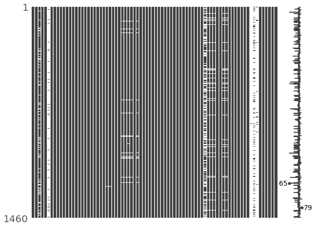
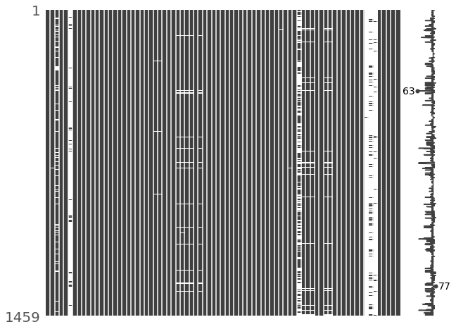
# 搜索缺失值
import missingno as msno
msno.matrix(df=df, figsize=(10,8))
# 查看相关性
#msno.heatmap(df=df,figsize=(10,8))
plot_missing(train)
plot_missing(test)
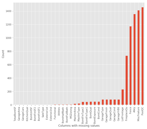
分析概要
以下是缺失比较多的feature
| Feature | Train miss | Test miss | Dispos |
|---|---|---|---|
| LotFrontage | 259 | 227 | 填个中位数吧 |
| Alley | 1369 | 1352 | 删除 |
| FireplaceQu | 690 | 730 | fireplaceQU 和 fireplaces 有关 缺失项貌似都是没有fireplace的 |
| PoolQC | 1453 | 1456 | 删除 |
| Fence | 1179 | 1169 | 删除 |
| MiscFeature | 1406 | 1408 | 删除 |
处理缺失值
# 删除缺失过多的feature
train = train.drop(['Alley', 'PoolQC', 'MiscFeature', 'Fence'], axis=1)
test = test.drop(['Alley', 'PoolQC', 'MiscFeature', 'Fence'], axis=1)
# FireplaceQu 缺失的都认为是没有的
train['FireplaceQu'] = train['FireplaceQu'].fillna('NA')
test['FireplaceQu'] = test['FireplaceQu'].fillna('NA')
# 填充其他缺失值
def fill_missing_values(df):
    # 查找缺失值
    missing = df.isnull().sum()
    missing = missing[missing > 0]

    for column in missing.index:
        # 类型为 object 的填众数
        if df[column].dtype == 'object':
            df[column].fillna(df[column].value_counts().index[0], inplace=True)
        # 其他类型填中位数
        else:
            df[column].fillna(df[column].median(), inplace=True)
fill_missing_values(train)
train.isnull().sum().max()
0
fill_missing_values(test)
test.isnull().sum().max()
0
好的,已经没有缺失数据了。
整理 description 文件
数据描述文件记录了所有特征所代表的含义,其中许多特征是字符串,现在我们要整理为个字典,便于我们查询。
description_dict = {}
with open('/data_description.txt','r') as description:
    description_data = description.read()
    description.close()

description_data = description_data.split('\n')
for i in description_data:
    if ':' in i:
        key = i.split(':')[0]
        description_dict[key] = []
    elif i.split() and '       ' in i:
        value = i.split()[0]
        description_dict[key].append(value)

print(description_dict)
{'MSSubClass': ['20', '30', '40', '45', '50', '60', '70', '75', '80', '85', '90', '120', '150', '160', '180', '190'], 'MSZoning': ['A', 'C', 'FV', 'I', 'RH', 'RL', 'RP', 'RM'], 'LotFrontage': [], 'LotArea': [], 'Street': ['Grvl', 'Pave'], 'Alley': ['Grvl', 'Pave', 'NA'], 'LotShape': ['Reg', 'IR1', 'IR2', 'IR3'], 'LandContour': ['Lvl', 'Bnk', 'HLS', 'Low'], 'Utilities': ['AllPub', 'NoSewr', 'NoSeWa', 'ELO'], 'LotConfig': ['Inside', 'Corner', 'CulDSac', 'FR2', 'FR3'], 'LandSlope': ['Gtl', 'Mod', 'Sev'], 'Neighborhood': ['Blmngtn', 'Blueste', 'BrDale', 'BrkSide', 'ClearCr', 'CollgCr', 'Crawfor', 'Edwards', 'Gilbert', 'IDOTRR', 'MeadowV', 'Mitchel', 'Names', 'NoRidge', 'NPkVill', 'NridgHt', 'NWAmes', 'OldTown', 'SWISU', 'Sawyer', 'SawyerW', 'Somerst', 'StoneBr', 'Timber', 'Veenker'], 'Condition1': ['Artery', 'Feedr', 'Norm', 'RRNn', 'RRAn', 'PosN', 'PosA', 'RRNe', 'RRAe'], 'Condition2': ['Artery', 'Feedr', 'Norm', 'RRNn', 'RRAn', 'PosN', 'PosA', 'RRNe', 'RRAe'], 'BldgType': ['1Fam', '2FmCon', 'Duplx', 'TwnhsE', 'TwnhsI'], 'HouseStyle': ['1Story'], ' 1.5Fin\tOne and one-half story': [], ' 1.5Unf\tOne and one-half story': ['2Story'], ' 2.5Fin\tTwo and one-half story': [], ' 2.5Unf\tTwo and one-half story': ['SFoyer', 'SLvl'], 'OverallQual': ['10', '9', '8', '7', '6', '5', '4', '3', '2', '1'], 'OverallCond': ['10', '9', '8', '7', '6', '5', '4', '3', '2', '1'], 'YearBuilt': [], 'YearRemodAdd': [], 'RoofStyle': ['Flat', 'Gable', 'Gambrel', 'Hip', 'Mansard', 'Shed'], 'RoofMatl': ['ClyTile', 'CompShg', 'Membran', 'Metal', 'Roll', 'Tar&Grv', 'WdShake', 'WdShngl'], 'Exterior1st': ['AsbShng', 'AsphShn', 'BrkComm', 'BrkFace', 'CBlock', 'CemntBd', 'HdBoard', 'ImStucc', 'MetalSd', 'Other', 'Plywood', 'PreCast', 'Stone', 'Stucco', 'VinylSd', 'Wd', 'WdShing'], 'Exterior2nd': ['AsbShng', 'AsphShn', 'BrkComm', 'BrkFace', 'CBlock', 'CemntBd', 'HdBoard', 'ImStucc', 'MetalSd', 'Other', 'Plywood', 'PreCast', 'Stone', 'Stucco', 'VinylSd', 'Wd', 'WdShing'], 'MasVnrType': ['BrkCmn', 'BrkFace', 'CBlock', 'None', 'Stone'], 'MasVnrArea': [], 'ExterQual': ['Ex', 'Gd', 'TA', 'Fa', 'Po'], 'ExterCond': ['Ex', 'Gd', 'TA', 'Fa', 'Po'], 'Foundation': ['BrkTil', 'CBlock', 'PConc', 'Slab', 'Stone', 'Wood'], 'BsmtQual': ['Ex', 'Gd', 'TA', 'Fa', 'Po', 'NA'], 'BsmtCond': ['Ex', 'Gd', 'TA', 'Fa', 'Po', 'NA'], 'BsmtExposure': ['Gd', 'Av', 'Mn', 'No', 'NA'], 'BsmtFinType1': ['GLQ', 'ALQ', 'BLQ', 'Rec', 'LwQ', 'Unf', 'NA'], 'BsmtFinSF1': [], 'BsmtFinType2': ['GLQ', 'ALQ', 'BLQ', 'Rec', 'LwQ', 'Unf', 'NA'], 'BsmtFinSF2': [], 'BsmtUnfSF': [], 'TotalBsmtSF': [], 'Heating': ['Floor', 'GasA', 'GasW', 'Grav', 'OthW', 'Wall'], 'HeatingQC': ['Ex', 'Gd', 'TA', 'Fa', 'Po'], 'CentralAir': ['N', 'Y'], 'Electrical': ['SBrkr', 'FuseA', 'FuseF', 'FuseP', 'Mix'], '1stFlrSF': [], '2ndFlrSF': [], 'LowQualFinSF': [], 'GrLivArea': [], 'BsmtFullBath': [], 'BsmtHalfBath': [], 'FullBath': [], 'HalfBath': [], 'Bedroom': [], 'Kitchen': [], 'KitchenQual': ['Ex', 'Gd', 'TA', 'Fa', 'Po'], 'TotRmsAbvGrd': [], 'Functional': ['Typ', 'Min1', 'Min2', 'Mod', 'Maj1', 'Maj2', 'Sev', 'Sal'], 'Fireplaces': [], 'FireplaceQu': ['Ex', 'Gd', 'TA', 'Fa', 'Po', 'NA'], 'GarageType': ['2Types', 'Attchd', 'Basment', 'BuiltIn', 'CarPort', 'Detchd', 'NA'], 'GarageYrBlt': [], 'GarageFinish': ['Fin', 'RFn', 'Unf', 'NA'], 'GarageCars': [], 'GarageArea': [], 'GarageQual': ['Ex', 'Gd', 'TA', 'Fa', 'Po', 'NA'], 'GarageCond': ['Ex', 'Gd', 'TA', 'Fa', 'Po', 'NA'], 'PavedDrive': ['Y', 'P', 'N'], 'WoodDeckSF': [], 'OpenPorchSF': [], 'EnclosedPorch': [], '3SsnPorch': [], 'ScreenPorch': [], 'PoolArea': [], 'PoolQC': ['Ex', 'Gd', 'TA', 'Fa', 'NA'], 'Fence': ['GdPrv', 'MnPrv', 'GdWo', 'MnWw', 'NA'], 'MiscFeature': ['Elev', 'Gar2', 'Othr', 'Shed', 'TenC', 'NA'], 'MiscVal': [], 'MoSold': [], 'YrSold': [], 'SaleType': ['WD', 'CWD', 'VWD', 'New', 'COD', 'Con', 'ConLw', 'ConLI', 'ConLD', 'Oth'], 'SaleCondition': ['Normal', 'Abnorml', 'AdjLand', 'Alloca', 'Family', 'Partial']}
字符串类型的 feature 重编码
# 这个函数的作用是得到数据集中非数字的feature column
def get_object_column(df):
    object_column = []
    for column in df.columns:
        if df[column].dtype == 'object':
            object_column.append(column)
    return object_column
#object_column = get_object_column(train)
# 这个函数的作用是把 description_dict 中的 value 转换为对应数字的字典
def generate_map(map_list, end_index=1):
    d = {}
    j = len(map_list) - end_index
    for i in map_list:
        d[i] = j
        j -= 1
    return d
def preprocess_order_feature(df):
    for i in get_object_column(df):
        order_map = generate_map(description_dict[i], 0)
        df[i] = df[i].map(order_map)
        df[i] = df[i].fillna(0)
    return df
train = preprocess_order_feature(train)
test = preprocess_order_feature(test)
观察数据
train.describe()
| MSSubClass | MSZoning | LotFrontage | LotArea | Street | LotShape | LandContour | Utilities | LotConfig | LandSlope | Neighborhood | Condition1 | Condition2 | BldgType | HouseStyle | OverallQual | OverallCond | YearBuilt | YearRemodAdd | RoofStyle | RoofMatl | Exterior1st | Exterior2nd | MasVnrType | MasVnrArea | ExterQual | ExterCond | Foundation | BsmtQual | BsmtCond | BsmtExposure | BsmtFinType1 | BsmtFinSF1 | BsmtFinType2 | BsmtFinSF2 | BsmtUnfSF | TotalBsmtSF | Heating | HeatingQC | CentralAir | Electrical | 1stFlrSF | 2ndFlrSF | LowQualFinSF | GrLivArea | BsmtFullBath | BsmtHalfBath | FullBath | HalfBath | BedroomAbvGr | KitchenAbvGr | KitchenQual | TotRmsAbvGrd | Functional | Fireplaces | FireplaceQu | GarageType | GarageYrBlt | GarageFinish | GarageCars | GarageArea | GarageQual | GarageCond | PavedDrive | WoodDeckSF | OpenPorchSF | EnclosedPorch | 3SsnPorch | ScreenPorch | PoolArea | MiscVal | MoSold | YrSold | SaleType | SaleCondition | SalePrice | |
|---|---|---|---|---|---|---|---|---|---|---|---|---|---|---|---|---|---|---|---|---|---|---|---|---|---|---|---|---|---|---|---|---|---|---|---|---|---|---|---|---|---|---|---|---|---|---|---|---|---|---|---|---|---|---|---|---|---|---|---|---|---|---|---|---|---|---|---|---|---|---|---|---|---|---|---|---|
| count | 1460.000000 | 1460.000000 | 1460.000000 | 1460.000000 | 1460.000000 | 1460.000000 | 1460.000000 | 1460.000000 | 1460.000000 | 1460.000000 | 1460.000000 | 1460.000000 | 1460.000000 | 1460.000000 | 1460.000000 | 1460.000000 | 1460.000000 | 1460.000000 | 1460.000000 | 1460.000000 | 1460.000000 | 1460.000000 | 1460.000000 | 1460.000000 | 1460.000000 | 1460.00000 | 1460.000000 | 1460.000000 | 1460.000000 | 1460.000000 | 1460.000000 | 1460.000000 | 1460.000000 | 1460.000000 | 1460.000000 | 1460.000000 | 1460.000000 | 1460.000000 | 1460.000000 | 1460.000000 | 1460.000000 | 1460.000000 | 1460.000000 | 1460.000000 | 1460.000000 | 1460.000000 | 1460.000000 | 1460.000000 | 1460.000000 | 1460.000000 | 1460.000000 | 1460.000000 | 1460.000000 | 1460.000000 | 1460.000000 | 1460.000000 | 1460.000000 | 1460.000000 | 1460.000000 | 1460.000000 | 1460.000000 | 1460.000000 | 1460.000000 | 1460.000000 | 1460.000000 | 1460.000000 | 1460.000000 | 1460.000000 | 1460.000000 | 1460.000000 | 1460.000000 | 1460.000000 | 1460.000000 | 1460.000000 | 1460.000000 | 1460.000000 |
| mean | 56.897260 | 2.825342 | 69.863699 | 10516.828082 | 1.004110 | 3.591781 | 3.814384 | 3.998630 | 4.583562 | 2.937671 | 10.747945 | 6.969178 | 6.993151 | 4.334247 | 0.497260 | 6.099315 | 5.575342 | 1971.267808 | 1984.865753 | 4.589726 | 6.924658 | 5.958904 | 5.271918 | 2.552740 | 103.117123 | 3.39589 | 3.083562 | 4.603425 | 4.565068 | 4.010959 | 2.656164 | 4.571233 | 443.639726 | 2.273288 | 46.549315 | 567.240411 | 1057.429452 | 4.963699 | 4.145205 | 1.065068 | 4.889726 | 1162.626712 | 346.992466 | 5.844521 | 1515.463699 | 0.425342 | 0.057534 | 1.565068 | 0.382877 | 2.866438 | 1.046575 | 3.511644 | 6.517808 | 7.841781 | 0.613014 | 2.825342 | 4.791781 | 1978.589041 | 2.771233 | 1.767123 | 472.980137 | 3.976712 | 3.975342 | 2.856164 | 94.244521 | 46.660274 | 21.954110 | 3.409589 | 15.060959 | 2.758904 | 43.489041 | 6.321918 | 2007.815753 | 9.509589 | 5.417808 | 180921.195890 |
| std | 42.300571 | 1.020174 | 22.027677 | 9981.264932 | 0.063996 | 0.582296 | 0.606509 | 0.052342 | 0.773448 | 0.276232 | 7.565716 | 0.878349 | 0.248272 | 1.555218 | 0.500164 | 1.382997 | 1.112799 | 30.202904 | 20.645407 | 0.834998 | 0.599127 | 4.426038 | 4.263353 | 1.046204 | 180.731373 | 0.57428 | 0.351054 | 0.722394 | 0.678071 | 0.284178 | 1.039123 | 2.070649 | 456.098091 | 0.869859 | 161.319273 | 441.866955 | 438.705324 | 0.295124 | 0.959501 | 0.246731 | 0.394658 | 386.587738 | 436.528436 | 48.623081 | 525.480383 | 0.518911 | 0.238753 | 0.550916 | 0.502885 | 0.815778 | 0.220338 | 0.663760 | 1.625393 | 0.667698 | 0.644666 | 1.810877 | 1.759864 | 23.997022 | 0.811835 | 0.747315 | 213.804841 | 0.241665 | 0.232860 | 0.496592 | 125.338794 | 66.256028 | 61.119149 | 29.317331 | 55.757415 | 40.177307 | 496.123024 | 2.703626 | 1.328095 | 1.368616 | 1.475209 | 79442.502883 |
| min | 20.000000 | 0.000000 | 21.000000 | 1300.000000 | 1.000000 | 1.000000 | 1.000000 | 2.000000 | 1.000000 | 1.000000 | 0.000000 | 1.000000 | 1.000000 | 0.000000 | 0.000000 | 1.000000 | 1.000000 | 1872.000000 | 1950.000000 | 1.000000 | 1.000000 | 0.000000 | 0.000000 | 1.000000 | 0.000000 | 2.00000 | 1.000000 | 1.000000 | 3.000000 | 2.000000 | 2.000000 | 2.000000 | 0.000000 | 2.000000 | 0.000000 | 0.000000 | 0.000000 | 1.000000 | 1.000000 | 1.000000 | 1.000000 | 334.000000 | 0.000000 | 0.000000 | 334.000000 | 0.000000 | 0.000000 | 0.000000 | 0.000000 | 0.000000 | 0.000000 | 2.000000 | 2.000000 | 2.000000 | 0.000000 | 1.000000 | 2.000000 | 1900.000000 | 2.000000 | 0.000000 | 0.000000 | 2.000000 | 2.000000 | 1.000000 | 0.000000 | 0.000000 | 0.000000 | 0.000000 | 0.000000 | 0.000000 | 0.000000 | 1.000000 | 2006.000000 | 1.000000 | 1.000000 | 34900.000000 |
| 25% | 20.000000 | 3.000000 | 60.000000 | 7553.500000 | 1.000000 | 3.000000 | 4.000000 | 4.000000 | 4.000000 | 3.000000 | 4.000000 | 7.000000 | 7.000000 | 5.000000 | 0.000000 | 5.000000 | 5.000000 | 1954.000000 | 1967.000000 | 5.000000 | 7.000000 | 3.000000 | 3.000000 | 2.000000 | 0.000000 | 3.00000 | 3.000000 | 4.000000 | 4.000000 | 4.000000 | 2.000000 | 2.000000 | 0.000000 | 2.000000 | 0.000000 | 223.000000 | 795.750000 | 5.000000 | 3.000000 | 1.000000 | 5.000000 | 882.000000 | 0.000000 | 0.000000 | 1129.500000 | 0.000000 | 0.000000 | 1.000000 | 0.000000 | 2.000000 | 1.000000 | 3.000000 | 5.000000 | 8.000000 | 0.000000 | 1.000000 | 2.000000 | 1962.000000 | 2.000000 | 1.000000 | 334.500000 | 4.000000 | 4.000000 | 3.000000 | 0.000000 | 0.000000 | 0.000000 | 0.000000 | 0.000000 | 0.000000 | 0.000000 | 5.000000 | 2007.000000 | 10.000000 | 6.000000 | 129975.000000 |
| 50% | 50.000000 | 3.000000 | 69.000000 | 9478.500000 | 1.000000 | 4.000000 | 4.000000 | 4.000000 | 5.000000 | 3.000000 | 10.000000 | 7.000000 | 7.000000 | 5.000000 | 0.000000 | 6.000000 | 5.000000 | 1973.000000 | 1994.000000 | 5.000000 | 7.000000 | 3.000000 | 3.000000 | 2.000000 | 0.000000 | 3.00000 | 3.000000 | 5.000000 | 5.000000 | 4.000000 | 2.000000 | 5.000000 | 383.500000 | 2.000000 | 0.000000 | 477.500000 | 991.500000 | 5.000000 | 5.000000 | 1.000000 | 5.000000 | 1087.000000 | 0.000000 | 0.000000 | 1464.000000 | 0.000000 | 0.000000 | 2.000000 | 0.000000 | 3.000000 | 1.000000 | 3.000000 | 6.000000 | 8.000000 | 1.000000 | 3.000000 | 6.000000 | 1980.000000 | 3.000000 | 2.000000 | 480.000000 | 4.000000 | 4.000000 | 3.000000 | 0.000000 | 25.000000 | 0.000000 | 0.000000 | 0.000000 | 0.000000 | 0.000000 | 6.000000 | 2008.000000 | 10.000000 | 6.000000 | 163000.000000 |
| 75% | 70.000000 | 3.000000 | 79.000000 | 11601.500000 | 1.000000 | 4.000000 | 4.000000 | 4.000000 | 5.000000 | 3.000000 | 18.000000 | 7.000000 | 7.000000 | 5.000000 | 1.000000 | 7.000000 | 6.000000 | 2000.000000 | 2004.000000 | 5.000000 | 7.000000 | 9.000000 | 9.000000 | 4.000000 | 164.250000 | 4.00000 | 3.000000 | 5.000000 | 5.000000 | 4.000000 | 3.000000 | 7.000000 | 712.250000 | 2.000000 | 0.000000 | 808.000000 | 1298.250000 | 5.000000 | 5.000000 | 1.000000 | 5.000000 | 1391.250000 | 728.000000 | 0.000000 | 1776.750000 | 1.000000 | 0.000000 | 2.000000 | 1.000000 | 3.000000 | 1.000000 | 4.000000 | 7.000000 | 8.000000 | 1.000000 | 5.000000 | 6.000000 | 2001.000000 | 3.000000 | 2.000000 | 576.000000 | 4.000000 | 4.000000 | 3.000000 | 168.000000 | 68.000000 | 0.000000 | 0.000000 | 0.000000 | 0.000000 | 0.000000 | 8.000000 | 2009.000000 | 10.000000 | 6.000000 | 214000.000000 |
| max | 190.000000 | 6.000000 | 313.000000 | 215245.000000 | 2.000000 | 4.000000 | 4.000000 | 4.000000 | 5.000000 | 3.000000 | 25.000000 | 9.000000 | 9.000000 | 5.000000 | 1.000000 | 10.000000 | 9.000000 | 2010.000000 | 2010.000000 | 6.000000 | 8.000000 | 17.000000 | 17.000000 | 5.000000 | 1600.000000 | 5.00000 | 5.000000 | 6.000000 | 6.000000 | 5.000000 | 5.000000 | 7.000000 | 5644.000000 | 7.000000 | 1474.000000 | 2336.000000 | 6110.000000 | 6.000000 | 5.000000 | 2.000000 | 5.000000 | 4692.000000 | 2065.000000 | 572.000000 | 5642.000000 | 3.000000 | 2.000000 | 3.000000 | 2.000000 | 8.000000 | 3.000000 | 5.000000 | 14.000000 | 8.000000 | 3.000000 | 6.000000 | 7.000000 | 2010.000000 | 4.000000 | 4.000000 | 1418.000000 | 6.000000 | 6.000000 | 3.000000 | 857.000000 | 547.000000 | 552.000000 | 508.000000 | 480.000000 | 738.000000 | 15500.000000 | 12.000000 | 2010.000000 | 10.000000 | 6.000000 | 755000.000000 |
观察 feature 之间的相关性
corr_mat = train[["SalePrice","MSSubClass","MSZoning","LotFrontage","LotArea", "BldgType",
                       "OverallQual", "OverallCond","YearBuilt", "BedroomAbvGr", "PoolArea", "GarageArea",
                       "SaleType", "MoSold"]].corr()
# corr_mat = train.corr()
f, ax = plt.subplots(figsize=(16, 8))
sns.heatmap(corr_mat, vmax=1 , square=True)
<matplotlib.axes._subplots.AxesSubplot at 0x7fb6c086fa20>
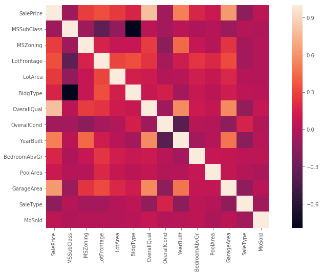
观察热力图,颜色越浅相关性越大。关于热力图-> this video.
观察年限和售价的规律
f, ax = plt.subplots(figsize=(16, 8))
sns.lineplot(x='YearBuilt', y='SalePrice', data=train)
<matplotlib.axes._subplots.AxesSubplot at 0x7fb6a5211320>
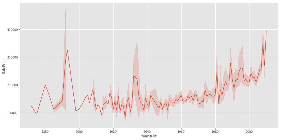
在二十世纪的时候价格增长迅速。
综合质量和售价有明显的相关性
f, ax = plt.subplots(figsize=(12, 8))
sns.lineplot(x='OverallQual', y='SalePrice', color='green',data=train)
<matplotlib.axes._subplots.AxesSubplot at 0x7fb6a3e6d8d0>
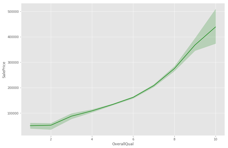
我们可以看到,随着房屋整体质量的提高,销售价格快速上涨,这是非常合理的。
观察售价
f, ax = plt.subplots(figsize=(10, 6))
sns.distplot(train['SalePrice'])
<matplotlib.axes._subplots.AxesSubplot at 0x7fb6a25cdba8>
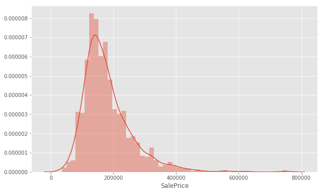
大部分的房屋售价在 100000 到 200000 之间。
构建预测模型
X = train.drop('SalePrice', axis=1)
y = np.ravel(np.array(train[['SalePrice']]))
print(y.shape)
y
(1460,)
array([208500, 181500, 223500, ..., 266500, 142125, 147500])
# Use train_test_split from sci-kit learn to segment our data into train and a local testset
X_train, X_test, y_train, y_test = train_test_split(X, y, test_size=0.2)
定义评估函数
评估函数基于预测值的对数与观察到的销售价格的对数之间的均方根误差(RMSE)。
def rmse(y, y_pred):
    return np.sqrt(mean_squared_error(np.log(y), np.log(y_pred)))
随机森林
random_forest = RandomForestRegressor(n_estimators=1200,
                                      max_depth=15,
                                      min_samples_split=5,
                                      min_samples_leaf=5,
                                      max_features=None,
                                      random_state=42,
                                      oob_score=True)
kf = KFold(n_splits=5)
y_pred = cross_val_score(random_forest, X, y, cv=kf)
y_pred.mean()
0.8500001566166802
random_forest.fit(X, y)
RandomForestRegressor(bootstrap=True, criterion='mse', max_depth=15,
max_features=None, max_leaf_nodes=None,
min_impurity_decrease=0.0, min_impurity_split=None,
min_samples_leaf=5, min_samples_split=5,
min_weight_fraction_leaf=0.0, n_estimators=1200,
n_jobs=None, oob_score=True, random_state=42, verbose=0,
warm_start=False)
rf_pred = random_forest.predict(test)
rf_pred
array([126945.71699684, 153924.56961003, 182182.80294353, ...,
156066.28489667, 117296.65091637, 224995.13115853])
XG Boost
xg_boost = XGBRegressor(learning_rate=0.01,
                        n_estimators=6000,
                        max_depth=4,
                        min_child_weight=1,
                        gamma=0.6,
                        subsample=0.7,
                        colsample_bytree=0.2,
                        objective='reg:linear',
                        nthread=-1,
                        scale_pos_weight=1,
                        seed=27,
                        reg_alpha=0.00006)

kf = KFold(n_splits=5)
y_pred = cross_val_score(xg_boost, X, y, cv=kf)
y_pred.mean()
[03:11:43] WARNING: /workspace/src/objective/regression_obj.cu:152: reg:linear is now deprecated in favor of reg:squarederror.
[03:11:51] WARNING: /workspace/src/objective/regression_obj.cu:152: reg:linear is now deprecated in favor of reg:squarederror.
[03:11:59] WARNING: /workspace/src/objective/regression_obj.cu:152: reg:linear is now deprecated in favor of reg:squarederror.
[03:12:06] WARNING: /workspace/src/objective/regression_obj.cu:152: reg:linear is now deprecated in favor of reg:squarederror.
[03:12:13] WARNING: /workspace/src/objective/regression_obj.cu:152: reg:linear is now deprecated in favor of reg:squarederror.
0.8959027545454475
xg_boost.fit(X, y)
[03:12:21] WARNING: /workspace/src/objective/regression_obj.cu:152: reg:linear is now deprecated in favor of reg:squarederror.
XGBRegressor(base_score=0.5, booster='gbtree', colsample_bylevel=1,
colsample_bynode=1, colsample_bytree=0.2, gamma=0.6,
importance_type='gain', learning_rate=0.01, max_delta_step=0,
max_depth=4, min_child_weight=1, missing=None, n_estimators=6000,
n_jobs=1, nthread=-1, objective='reg:linear', random_state=0,
reg_alpha=6e-05, reg_lambda=1, scale_pos_weight=1, seed=27,
silent=None, subsample=0.7, verbosity=1)
xgb_pred = xg_boost.predict(test)
xgb_pred
array([127263.77 , 163056.02 , 193208.25 , ..., 173218.75 , 115712.914,
211616.88 ], dtype=float32)
Gradient Boost Regressor(GBM)
g_boost = GradientBoostingRegressor(n_estimators=6000,
                                    learning_rate=0.01,
                                    max_depth=5,
                                    max_features='sqrt',
                                    min_samples_leaf=15,
                                    min_samples_split=10,
                                    loss='ls',
                                    random_state=42
                                    )

kf = KFold(n_splits=5)
y_pred = cross_val_score(g_boost, X, y, cv=kf)
y_pred.mean()
0.8905525972502479
g_boost.fit(X, y)
GradientBoostingRegressor(alpha=0.9, criterion='friedman_mse', init=None,
learning_rate=0.01, loss='ls', max_depth=5,
max_features='sqrt', max_leaf_nodes=None,
min_impurity_decrease=0.0, min_impurity_split=None,
min_samples_leaf=15, min_samples_split=10,
min_weight_fraction_leaf=0.0, n_estimators=6000,
n_iter_no_change=None, presort='auto',
random_state=42, subsample=1.0, tol=0.0001,
validation_fraction=0.1, verbose=0, warm_start=False)
gbm_pred = g_boost.predict(test)
gbm_pred
array([125909.87154943, 163184.8652622 , 187872.72372976, ...,
176429.22616544, 119620.23912638, 211953.00041747])
Light GBM
lightgbm = LGBMRegressor(objective='regression',
                         num_leaves=6,
                         learning_rate=0.01,
                         n_estimators=6400,
                         verbose=-1,
                         bagging_fraction=0.8,
                         bagging_freq=4,
                         bagging_seed=6,
                         feature_fraction=0.2,
                         feature_fraction_seed=7
                         )
kf = KFold(n_splits=5)
y_pred = cross_val_score(lightgbm, X, y, cv=kf)
y_pred.mean()
0.8881867437856128
lightgbm.fit(X,y)
LGBMRegressor(bagging_fraction=0.8, bagging_freq=4, bagging_seed=6,
boosting_type='gbdt', class_weight=None, colsample_bytree=1.0,
feature_fraction=0.2, feature_fraction_seed=7,
importance_type='split', learning_rate=0.01, max_depth=-1,
min_child_samples=20, min_child_weight=0.001, min_split_gain=0.0,
n_estimators=6400, n_jobs=-1, num_leaves=6,
objective='regression', random_state=None, reg_alpha=0.0,
reg_lambda=0.0, silent=True, subsample=1.0,
subsample_for_bin=200000, subsample_freq=0, verbose=-1)
lgb_pred = lightgbm.predict(test)
lgb_pred
array([124759.4703253 , 161206.70919126, 187680.444818 , ...,
168310.83365532, 123698.90457326, 206480.92047866])
Logistic Regression
logreg = LogisticRegression()
kf = KFold(n_splits=5)
y_pred = cross_val_score(logreg, X, y, cv=kf)
y_pred.mean()
logreg.fit(X, y)
/usr/local/lib/python3.6/dist-packages/sklearn/linear_model/logistic.py:432: FutureWarning: Default solver will be changed to 'lbfgs' in 0.22. Specify a solver to silence this warning.
FutureWarning)
/usr/local/lib/python3.6/dist-packages/sklearn/linear_model/logistic.py:469: FutureWarning: Default multi_class will be changed to 'auto' in 0.22. Specify the multi_class option to silence this warning.
"this warning.", FutureWarning)
/usr/local/lib/python3.6/dist-packages/sklearn/svm/base.py:929: ConvergenceWarning: Liblinear failed to converge, increase the number of iterations.
"the number of iterations.", ConvergenceWarning)
LogisticRegression(C=1.0, class_weight=None, dual=False, fit_intercept=True,
intercept_scaling=1, l1_ratio=None, max_iter=100,
multi_class='warn', n_jobs=None, penalty='l2',
random_state=None, solver='warn', tol=0.0001, verbose=0,
warm_start=False)
round(logreg.score(X, y) * 100, 2)
88.9
log_pred = logreg.predict(test)
log_pred
array([135500, 128950, 175000, ..., 133900, 190000, 187500])
模型的叠加
叠加(也称为元集成)是一种模型集成技术,用于组合来自多个预测模型的信息,生成性能更好的新模型。在这个项目中,我们使用名为vecstack的python包,它可以帮助我们对前面导入的模型进行堆栈。它实际上非常容易使用,可以查看文档了解更多信息。vecstack
models = [g_boost, xg_boost, lightgbm, random_forest]
Strain, S_test = stacking(models,
                          X_train,
                          y_train,
                          X_test,
                          regression=True,
                          mode='oof_pred_bag',
                          metric=rmse,
                          n_folds=5,
                          random_state=25,
                          verbose=2)
task: [regression]
metric: [rmse]
mode: [oof_pred_bag]
n_models: [4]
model 0: [GradientBoostingRegressor]
fold 0: [0.12653004]
fold 1: [0.13818165]
fold 2: [0.10747644]
fold 3: [0.14980732]
fold 4: [0.11127270]
----
MEAN: [0.12665363] + [0.01595833]
FULL: [0.12764756]
model 1: [XGBRegressor]
[03:23:54] WARNING: /workspace/src/objective/regression_obj.cu:152: reg:linear is now deprecated in favor of reg:squarederror.
fold 0: [0.11631560]
[03:24:00] WARNING: /workspace/src/objective/regression_obj.cu:152: reg:linear is now deprecated in favor of reg:squarederror.
fold 1: [0.14701253]
[03:24:06] WARNING: /workspace/src/objective/regression_obj.cu:152: reg:linear is now deprecated in favor of reg:squarederror.
fold 2: [0.10450330]
[03:24:12] WARNING: /workspace/src/objective/regression_obj.cu:152: reg:linear is now deprecated in favor of reg:squarederror.
fold 3: [0.14328067]
[03:24:18] WARNING: /workspace/src/objective/regression_obj.cu:152: reg:linear is now deprecated in favor of reg:squarederror.
fold 4: [0.10632026]
----
MEAN: [0.12348647] + [0.01817552]
FULL: [0.12481458]
model 2: [LGBMRegressor]
fold 0: [0.12668239]
fold 1: [0.14251415]
fold 2: [0.11409004]
fold 3: [0.15394461]
fold 4: [0.11576550]
----
MEAN: [0.13059934] + [0.01545902]
FULL: [0.13150292]
model 3: [RandomForestRegressor]
fold 0: [0.13803357]
fold 1: [0.16746496]
fold 2: [0.13370269]
fold 3: [0.17907099]
fold 4: [0.13625091]
----
MEAN: [0.15090463] + [0.01867560]
FULL: [0.15204350]
Strain, S_test
(array([[145154.57609501, 140247.640625 , 144708.92814448,
136304.80002144],
[441586.84575012, 453786.875 , 476049.8262998 ,
433615.5690085 ],
[205559.38156983, 199459.953125 , 204548.62741617,
189012.87710637],
...,
[229773.83814053, 245324.03125 , 222988.34529258,
233726.54189435],
[ 78529.68615301, 81706.46875 , 74919.86211206,
94651.91862458],
[126564.42955093, 118016.921875 , 131591.97464745,
134449.34870648]]),
array([[156946.11019358, 162235.903125 , 156274.58204718,
174271.19166786],
[168719.74644755, 171368.26875 , 172660.15892698,
168988.4858204 ],
[165875.73697659, 167827.703125 , 166511.09786993,
144720.7621456 ],
...,
[235105.18179731, 240780.803125 , 236012.18528746,
224310.44197611],
[311340.99357469, 306275.29375 , 305036.50098821,
319953.95931372],
[100400.26285948, 97430.8671875 , 97576.05463032,
109458.70614352]]))
# Initialize 2nd level model
xgb_lev2 = XGBRegressor(learning_rate=0.1,
                        n_estimators=500,
                        max_depth=3,
                        n_jobs=-1,
                        random_state=17
                       )

# Fit the 2nd level model on the output of level 1
xgb_lev2.fit(Strain, y_train)
[03:25:26] WARNING: /workspace/src/objective/regression_obj.cu:152: reg:linear is now deprecated in favor of reg:squarederror.
XGBRegressor(base_score=0.5, booster='gbtree', colsample_bylevel=1,
colsample_bynode=1, colsample_bytree=1, gamma=0,
importance_type='gain', learning_rate=0.1, max_delta_step=0,
max_depth=3, min_child_weight=1, missing=None, n_estimators=500,
n_jobs=-1, nthread=None, objective='reg:linear', random_state=17,
reg_alpha=0, reg_lambda=1, scale_pos_weight=1, seed=None,
silent=None, subsample=1, verbosity=1)
# Make predictions on the localized test set
stacked_pred = xgb_lev2.predict(S_test)
print("RMSE of Stacked Model: {}".format(rmse(y_test,stacked_pred)))
RMSE of Stacked Model: 0.12290530277450722
y1_pred_L1 = models[0].predict(test)
y2_pred_L1 = models[1].predict(test)
y3_pred_L1 = models[2].predict(test)
y4_pred_L1 = models[3].predict(test)
S_test_L1 = np.c_[y1_pred_L1, y2_pred_L1, y3_pred_L1, y4_pred_L1]
test_stacked_pred = xgb_lev2.predict(S_test_L1)
# Save the predictions in form of a dataframe
submission = pd.DataFrame()

submission['Id'] = np.array(test.index)
submission['SalePrice'] = test_stacked_pred
submission.to_csv('/submissionV2.csv', index=False)
混合较好得分的 submission
因为不知道最终的测试集合的正真数据是什么,只能一遍一遍提交去蒙,看到别人的方法是混合他人较好的提交去验证,尝试下看看。
submission_v1 = pd.read_csv('/House_price_submission_v44.csv')
submission_v2 = pd.read_csv('/submissionV19.csv')
submission_v3 = pd.read_csv('/blended_submission.csv')
final_blend = 0.5*submission_v1.SalePrice.values + 0.2*submission_v2.SalePrice.values + 0.3*submission_v3.SalePrice.values

blended_submission = pd.DataFrame()

blended_submission['Id'] = submission_v1.Id.values
blended_submission['SalePrice'] = final_blend
blended_submission.to_csv('/submissionV20.csv', index=False)
blended_submission

呃,就这样吧,最终和前十名差不到0.004。
用 Tensorfolw 试试
import math
import tensorflow as tf
from tensorflow.python.data import Dataset
from sklearn.model_selection import train_test_split
from sklearn import metrics
tf.logging.set_verbosity(tf.logging.ERROR)
correlation_dataframe = train.copy()
saleprice_corr = correlation_dataframe.corr()['SalePrice']
saleprice_corr = saleprice_corr[saleprice_corr > 0]
corr_feature = saleprice_corr.index
corr_feature
Index(['MSZoning', 'LotFrontage', 'LotArea', 'Utilities', 'BldgType',
'OverallQual', 'YearBuilt', 'YearRemodAdd', 'MasVnrType', 'MasVnrArea',
'ExterQual', 'ExterCond', 'BsmtQual', 'BsmtCond', 'BsmtExposure',
'BsmtFinType1', 'BsmtFinSF1', 'BsmtUnfSF', 'TotalBsmtSF', 'Heating',
'HeatingQC', 'Electrical', '1stFlrSF', '2ndFlrSF', 'GrLivArea',
'BsmtFullBath', 'FullBath', 'HalfBath', 'BedroomAbvGr', 'KitchenQual',
'TotRmsAbvGrd', 'Functional', 'Fireplaces', 'FireplaceQu', 'GarageType',
'GarageYrBlt', 'GarageFinish', 'GarageCars', 'GarageArea', 'GarageQual',
'GarageCond', 'PavedDrive', 'WoodDeckSF', 'OpenPorchSF', '3SsnPorch',
'ScreenPorch', 'PoolArea', 'MoSold', 'SalePrice'],
dtype='object')
def preprocess_feature(df, corr_feature):
    newdf = pd.DataFrame()
    for feature in corr_feature:
        newdf[feature] = df[feature]
    return newdf
X = preprocess_feature(train, corr_feature).drop('SalePrice', axis=1)
y = np.ravel(np.array(train[['SalePrice']]))
X.describe()
| MSZoning | LotFrontage | LotArea | Utilities | BldgType | OverallQual | YearBuilt | YearRemodAdd | MasVnrType | MasVnrArea | ExterQual | ExterCond | BsmtQual | BsmtCond | BsmtExposure | BsmtFinType1 | BsmtFinSF1 | BsmtUnfSF | TotalBsmtSF | Heating | HeatingQC | Electrical | 1stFlrSF | 2ndFlrSF | GrLivArea | BsmtFullBath | FullBath | HalfBath | BedroomAbvGr | KitchenQual | TotRmsAbvGrd | Functional | Fireplaces | FireplaceQu | GarageType | GarageYrBlt | GarageFinish | GarageCars | GarageArea | GarageQual | GarageCond | PavedDrive | WoodDeckSF | OpenPorchSF | 3SsnPorch | ScreenPorch | PoolArea | MoSold | |
|---|---|---|---|---|---|---|---|---|---|---|---|---|---|---|---|---|---|---|---|---|---|---|---|---|---|---|---|---|---|---|---|---|---|---|---|---|---|---|---|---|---|---|---|---|---|---|---|---|
| count | 1460.000000 | 1460.000000 | 1460.000000 | 1460.000000 | 1460.000000 | 1460.000000 | 1460.000000 | 1460.000000 | 1460.000000 | 1460.000000 | 1460.00000 | 1460.000000 | 1460.000000 | 1460.000000 | 1460.000000 | 1460.000000 | 1460.000000 | 1460.000000 | 1460.000000 | 1460.000000 | 1460.000000 | 1460.000000 | 1460.000000 | 1460.000000 | 1460.000000 | 1460.000000 | 1460.000000 | 1460.000000 | 1460.000000 | 1460.000000 | 1460.000000 | 1460.000000 | 1460.000000 | 1460.000000 | 1460.000000 | 1460.000000 | 1460.000000 | 1460.000000 | 1460.000000 | 1460.000000 | 1460.000000 | 1460.000000 | 1460.000000 | 1460.000000 | 1460.000000 | 1460.000000 | 1460.000000 | 1460.000000 |
| mean | 2.825342 | 69.863699 | 10516.828082 | 3.998630 | 4.334247 | 6.099315 | 1971.267808 | 1984.865753 | 2.552740 | 103.117123 | 3.39589 | 3.083562 | 4.565068 | 4.010959 | 2.656164 | 4.571233 | 443.639726 | 567.240411 | 1057.429452 | 4.963699 | 4.145205 | 4.889726 | 1162.626712 | 346.992466 | 1515.463699 | 0.425342 | 1.565068 | 0.382877 | 2.866438 | 3.511644 | 6.517808 | 7.841781 | 0.613014 | 2.825342 | 4.791781 | 1978.589041 | 2.771233 | 1.767123 | 472.980137 | 3.976712 | 3.975342 | 2.856164 | 94.244521 | 46.660274 | 3.409589 | 15.060959 | 2.758904 | 6.321918 |
| std | 1.020174 | 22.027677 | 9981.264932 | 0.052342 | 1.555218 | 1.382997 | 30.202904 | 20.645407 | 1.046204 | 180.731373 | 0.57428 | 0.351054 | 0.678071 | 0.284178 | 1.039123 | 2.070649 | 456.098091 | 441.866955 | 438.705324 | 0.295124 | 0.959501 | 0.394658 | 386.587738 | 436.528436 | 525.480383 | 0.518911 | 0.550916 | 0.502885 | 0.815778 | 0.663760 | 1.625393 | 0.667698 | 0.644666 | 1.810877 | 1.759864 | 23.997022 | 0.811835 | 0.747315 | 213.804841 | 0.241665 | 0.232860 | 0.496592 | 125.338794 | 66.256028 | 29.317331 | 55.757415 | 40.177307 | 2.703626 |
| min | 0.000000 | 21.000000 | 1300.000000 | 2.000000 | 0.000000 | 1.000000 | 1872.000000 | 1950.000000 | 1.000000 | 0.000000 | 2.00000 | 1.000000 | 3.000000 | 2.000000 | 2.000000 | 2.000000 | 0.000000 | 0.000000 | 0.000000 | 1.000000 | 1.000000 | 1.000000 | 334.000000 | 0.000000 | 334.000000 | 0.000000 | 0.000000 | 0.000000 | 0.000000 | 2.000000 | 2.000000 | 2.000000 | 0.000000 | 1.000000 | 2.000000 | 1900.000000 | 2.000000 | 0.000000 | 0.000000 | 2.000000 | 2.000000 | 1.000000 | 0.000000 | 0.000000 | 0.000000 | 0.000000 | 0.000000 | 1.000000 |
| 25% | 3.000000 | 60.000000 | 7553.500000 | 4.000000 | 5.000000 | 5.000000 | 1954.000000 | 1967.000000 | 2.000000 | 0.000000 | 3.00000 | 3.000000 | 4.000000 | 4.000000 | 2.000000 | 2.000000 | 0.000000 | 223.000000 | 795.750000 | 5.000000 | 3.000000 | 5.000000 | 882.000000 | 0.000000 | 1129.500000 | 0.000000 | 1.000000 | 0.000000 | 2.000000 | 3.000000 | 5.000000 | 8.000000 | 0.000000 | 1.000000 | 2.000000 | 1962.000000 | 2.000000 | 1.000000 | 334.500000 | 4.000000 | 4.000000 | 3.000000 | 0.000000 | 0.000000 | 0.000000 | 0.000000 | 0.000000 | 5.000000 |
| 50% | 3.000000 | 69.000000 | 9478.500000 | 4.000000 | 5.000000 | 6.000000 | 1973.000000 | 1994.000000 | 2.000000 | 0.000000 | 3.00000 | 3.000000 | 5.000000 | 4.000000 | 2.000000 | 5.000000 | 383.500000 | 477.500000 | 991.500000 | 5.000000 | 5.000000 | 5.000000 | 1087.000000 | 0.000000 | 1464.000000 | 0.000000 | 2.000000 | 0.000000 | 3.000000 | 3.000000 | 6.000000 | 8.000000 | 1.000000 | 3.000000 | 6.000000 | 1980.000000 | 3.000000 | 2.000000 | 480.000000 | 4.000000 | 4.000000 | 3.000000 | 0.000000 | 25.000000 | 0.000000 | 0.000000 | 0.000000 | 6.000000 |
| 75% | 3.000000 | 79.000000 | 11601.500000 | 4.000000 | 5.000000 | 7.000000 | 2000.000000 | 2004.000000 | 4.000000 | 164.250000 | 4.00000 | 3.000000 | 5.000000 | 4.000000 | 3.000000 | 7.000000 | 712.250000 | 808.000000 | 1298.250000 | 5.000000 | 5.000000 | 5.000000 | 1391.250000 | 728.000000 | 1776.750000 | 1.000000 | 2.000000 | 1.000000 | 3.000000 | 4.000000 | 7.000000 | 8.000000 | 1.000000 | 5.000000 | 6.000000 | 2001.000000 | 3.000000 | 2.000000 | 576.000000 | 4.000000 | 4.000000 | 3.000000 | 168.000000 | 68.000000 | 0.000000 | 0.000000 | 0.000000 | 8.000000 |
| max | 6.000000 | 313.000000 | 215245.000000 | 4.000000 | 5.000000 | 10.000000 | 2010.000000 | 2010.000000 | 5.000000 | 1600.000000 | 5.00000 | 5.000000 | 6.000000 | 5.000000 | 5.000000 | 7.000000 | 5644.000000 | 2336.000000 | 6110.000000 | 6.000000 | 5.000000 | 5.000000 | 4692.000000 | 2065.000000 | 5642.000000 | 3.000000 | 3.000000 | 2.000000 | 8.000000 | 5.000000 | 14.000000 | 8.000000 | 3.000000 | 6.000000 | 7.000000 | 2010.000000 | 4.000000 | 4.000000 | 1418.000000 | 6.000000 | 6.000000 | 3.000000 | 857.000000 | 547.000000 | 508.000000 | 480.000000 | 738.000000 | 12.000000 |
def my_input_fn(features, targets, batch_size=1, shuffle=True, num_epochs=None):
    features = {key: np.array(value) for key, value in dict(features).items()}

    ds = Dataset.from_tensor_slices((features, targets))
    ds = ds.batch(batch_size).repeat(num_epochs)

    if shuffle:
        ds = ds.shuffle(10000)

    features, labels = ds.make_one_shot_iterator().get_next()
    return features, labels
def construct_feature_columns(input_features):
    """构造TensorFlow特征列
        参数:
            input_features:要使用的数字输入特性的名称。
        返回:
            一个 feature columns 集合
    """
    return set([tf.feature_column.numeric_column(my_feature)
                for my_feature in input_features])
def train_model(
learning_rate,
strps,
batch_size,
training_examples,
training_targets,
validation_examples,
validation_targets):
"""训练多元特征的线性回归模型
除训练外,此功能还打印训练进度信息,
以及随着时间的推移而失去的训练和验证。
参数:
learning_rate:一个float,表示学习率
steps:一个非零的int,训练步骤的总数。训练步骤
由使用单个批处理的向前和向后传递组成。
batch_size:一个非零的int
training_example: DataFrame 包含一个或多个列
' california_housing_dataframe '作为训练的输入feature
training_targets:一个' DataFrame ',它只包含一列
' california_housing_dataframe '作为训练的目标。
validation_example: ' DataFrame '包含一个或多个列
' california_housing_dataframe '作为验证的输入feature
validation_targets: ' DataFrame ',仅包含来自其中的一列
' california_housing_dataframe '作为验证的目标。
返回:
在训练数据上训练的“线性回归器”对象
"""
periods = 10
steps_per_period = strps / periods
# 创建一个线性回归对象
my_optimizer = tf.train.GradientDescentOptimizer(learning_rate=learning_rate)
my_optimizer = tf.contrib.estimator.clip_gradients_by_norm(my_optimizer, 5.0)
linear_regressor = tf.estimator.LinearRegressor(
feature_columns=construct_feature_columns(training_examples),
optimizer=my_optimizer
)
# 创建输入函数
training_input_fn = lambda: my_input_fn(
training_examples,
training_targets,
batch_size=batch_size)
predict_training_input_fn = lambda: my_input_fn(
training_examples,
training_targets,
num_epochs=1,
shuffle=False)
predict_validation_input_fn = lambda: my_input_fn(
validation_examples,
validation_targets,
num_epochs=1,
shuffle=False)
#训练模型,但要在循环中进行,这样我们才能定期评估
#损失指标
print("Training model...")
print("RMSE (on training data):")
training_rmse = []
validation_rmse = []
for period in range (0, periods):
# Train the model, starting from the prior state.
linear_regressor.train(
input_fn=training_input_fn,
steps=steps_per_period,
)
# Take a break and compute predictions.
training_predictions = linear_regressor.predict(input_fn=predict_training_input_fn)
training_predictions = np.array([item['predictions'][0] for item in training_predictions])
validation_predictions = linear_regressor.predict(input_fn=predict_validation_input_fn)
validation_predictions = np.array([item['predictions'][0] for item in validation_predictions])
# Compute training and validation loss.
training_root_mean_squared_error = math.sqrt(
metrics.mean_squared_error(training_predictions, training_targets))
validation_root_mean_squared_error = math.sqrt(
metrics.mean_squared_error(validation_predictions, validation_targets))
# Occasionally print the current loss.
print(" period %02d : %0.2f" % (period, training_root_mean_squared_error))
# Add the loss metrics from this period to our list.
training_rmse.append(training_root_mean_squared_error)
validation_rmse.append(validation_root_mean_squared_error)
print("Model training finished.")
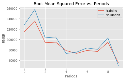
# Output a graph of loss metrics over periods.
plt.ylabel("RMSE")
plt.xlabel("Periods")
plt.title("Root Mean Squared Error vs. Periods")
plt.tight_layout()
plt.plot(training_rmse, label="training")
plt.plot(validation_rmse, label="validation")
plt.legend()
return linear_regressor
linear_regressor = train_model(
    learning_rate=0.5,
    strps=200,
    batch_size=5,
    training_examples=X_train,
    training_targets=y_train,
    validation_examples=X_test,
    validation_targets=y_test)
Training model...
RMSE (on training data):
period 00 : 115236.06
period 01 : 135729.29
period 02 : 94007.13
period 03 : 94940.56
period 04 : 78776.40
period 05 : 73407.86
period 06 : 79100.02
period 07 : 76995.32
period 08 : 94657.55
period 09 : 55721.83
Model training finished.
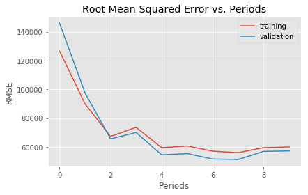
linear_regressor2 = train_model(
    learning_rate=0.25,
    strps=500,
    batch_size=5,
    training_examples=X_train,
    training_targets=y_train,
    validation_examples=X_test,
    validation_targets=y_test)
Training model...
RMSE (on training data):
period 00 : 126663.18
period 01 : 89900.76
period 02 : 67300.53
period 03 : 73597.13
period 04 : 59429.95
period 05 : 60645.34
period 06 : 57056.42
period 07 : 55974.51
period 08 : 59490.64
period 09 : 59963.44
Model training finished.
predict_test_input_fn = lambda: my_input_fn(
      test,
      test,
      num_epochs=1,
      shuffle=False)

test_predictions = linear_regressor.predict(input_fn=predict_test_input_fn)
test_predictions = np.array([item['predictions'][0] for item in test_predictions])
test_predictions
array([152403.8 , 178793.02, 186845.23, ..., 203018.39, 142496.02,
197809.12], dtype=float32)
就先这样吧。