ex5-bias vs variance

AndrewNg 机器学习习题ex5-bias vs variance

ex5data1.mat文件储存了大坝出水量的数据，由三部分组成：

训练集：X，y
交叉验证集：Xval，yval
测试集：Xtest，ytest

需要的头：

import numpy as np
import scipy.io as sio
import scipy.optimize as opt
import pandas as pd
import matplotlib.pyplot as plt
import seaborn as sns

数据预处理

画出训练集的散点图，给特征集加一列1.

def load_data():
    d = sio.loadmat('./data/ex5data1.mat')
    return map(np.ravel, [d['X'], d['y'], d['Xval'], d['yval'], d['Xtest'], d['ytest']])


X, y, Xval, yval, Xtest, ytest = load_data()
df = pd.DataFrame({'water_level': X, 'flow': y})
print(df.shape)
sns.lmplot('water_level', 'flow', data=df, fit_reg=False)
plt.show()

X, Xval, Xtest = [np.insert(x.reshape(x.shape[0], 1), 0, np.ones(x.shape[0]), axis=1) for x in (X, Xval, Xtest)]
# print(X, Xval, Xtest )

正则化

代价函数是：

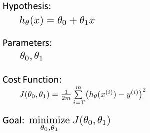
梯度下降：

$θ_{j} := θ_{j} - α \frac{\partial}{\partial θ_{j}} J (θ)$

正则化线性回归的代价函数为：

$J (θ) = \frac{1}{2 m} \sum_{i = 1}^{m} [({(h_{θ} (x^{(i)}) - y^{(i)})}^{2} + λ \sum_{j = 1}^{n} θ_{j}^{2})]$

如果我们要使用梯度下降法令这个代价函数最小化，因为我们未对 $θ_{0}$ 进行正则化，所以梯度下降算法将分两种情形：

$R e p e a t$ $u n t i l$ $c o n v e r g e n c e$ {

$θ_{0} := θ_{0} - a \frac{1}{m} \sum_{i = 1}^{m} ((h_{θ} (x^{(i)}) - y^{(i)}) x_{0}^{(i)})$

$θ_{j} := θ_{j} - a [\frac{1}{m} \sum_{i = 1}^{m} ((h_{θ} (x^{(i)}) - y^{(i)}) x_{j}^{(i)} + \frac{λ}{m} θ_{j}]$

$f o r$ $j = 1, 2, . . . n$

}

# 代价函数
def cost(theta, X, y):
    m = X.shape[0]
    inner = X @ theta - y  # R(m+1)
    # 1*m @ m*1 = 1*1 矩阵乘法
    # 一维矩阵的转置乘以它自己等于每个元素的平方和
    return inner.T @ inner / (2 * m)



print(cost(theta, X, y,))
# 303.9515255535976

# 梯度
def gradient(theta, X, y):
    m = X.shape[0]
    return X.T @ (X @ theta - y) / m  # (m, n).T @ (m, 1) -> (n, 1)


print(gradient(theta, X, y,))
# [-15.30301567 598.16741084]


# 正则化
def regularized_cost(theta, X, y, l=1):
    return cost(theta, X, y) + (l / (2 * X.shape[0])) * np.power(theta[1:], 2).sum()


def regularized_gradient(theta, X, y, l=1):
    m = X.shape[0]
    regularized_term = theta.copy()
    regularized_term[0] = 0
    regularized_term = (l / m) * regularized_term
    return gradient(theta, X, y) + regularized_term

print(regularized_gradient(theta, X, y, l=1))
# [-15.30301567 598.25074417]

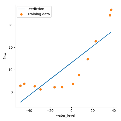
训练数据

正则化项 $λ = 0$

def linear_regression_np(theta, X, y, l=1):
    res = opt.fmin_tnc(func=regularized_cost, x0=theta, fprime=regularized_gradient, args=(X, y))
    return res


final_theta = linear_regression_np(theta, X, y)[0]
b = final_theta[0]
m = final_theta[1]

plt.scatter(X[:, 1], y, label="Training data")
plt.plot(X[:, 1], X[:, 1]*m + b, label='Prediction')
plt.legend(loc=2)
plt.show()

学习曲线

def plot_learning_curve(X, y, Xval, yval, l=0):
    training_cost, cv_cost = [], []  # 计算训练集的代价和交叉验证（cross validation）集的代价
    m = X.shape[0]
    for i in range(1, m + 1):
        res = linear_regression_np(theta, X[:i, :], y[:i], l=0)

        tc = regularized_cost(res[0], X[:i, :], y[:i], l=0)
        cv = regularized_cost(res[0], Xval, yval, l=0)

        training_cost.append(tc)
        cv_cost.append(cv)

    plt.plot(np.arange(1, m + 1), training_cost, label='training cost')
    plt.plot(np.arange(1, m + 1), cv_cost, label='cv cost')
    plt.legend(loc=1)


plot_learning_curve(X, y, Xval, yval, l=0)
plt.show()

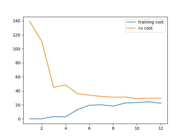
观察学习曲线发现拟合的不太好，欠拟合。很显然我们的模型不优秀，改为多项式特征尝试。

多项式特征

把特征扩展到8阶，然后归一化特征值。

def poly_features(x, power, as_ndarray=False):
    data = {'f{}'.format(i): np.power(x, i) for i in range(1, power + 1)}
    df = pd.DataFrame(data)
    return df.as_matrix() if as_ndarray else df


# 归一化特征值，减去平均数除以标准差
def normalize_feature(df):
    """Applies function along input axis(default 0) of DataFrame."""
    return df.apply(lambda column: (column - column.mean()) / column.std())


def prepare_poly_data(*args, power):
    """
    args: keep feeding in X, Xval, or Xtest
        will return in the same order
    """
    def prepare(x):
        # expand feature
        df = poly_features(x, power=power)

        # normalization
        ndarr = normalize_feature(df).as_matrix()

        # add intercept term
        return np.insert(ndarr, 0, np.ones(ndarr.shape[0]), axis=1)

    return [prepare(x) for x in args]

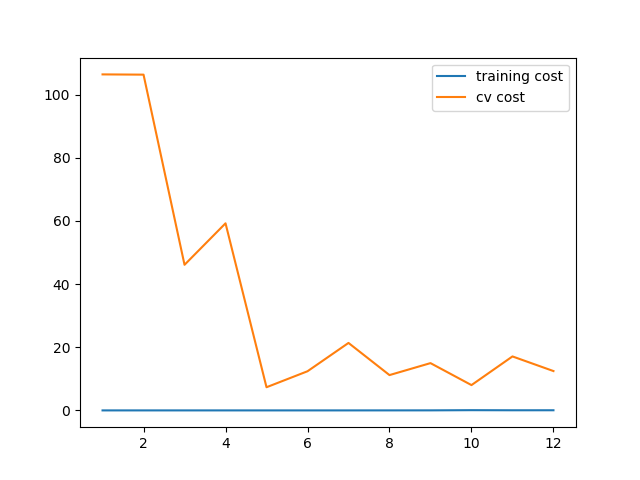
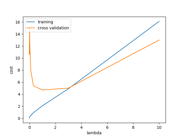
尝试不同的λ来观察学习曲线

X, y, Xval, yval, Xtest, ytest = load_data()
X_poly, Xval_poly, Xtest_poly= prepare_poly_data(X, Xval, Xtest, power=8)

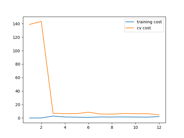
plot_learning_curve(X_poly, y, Xval_poly, yval, l=0)
plt.show()
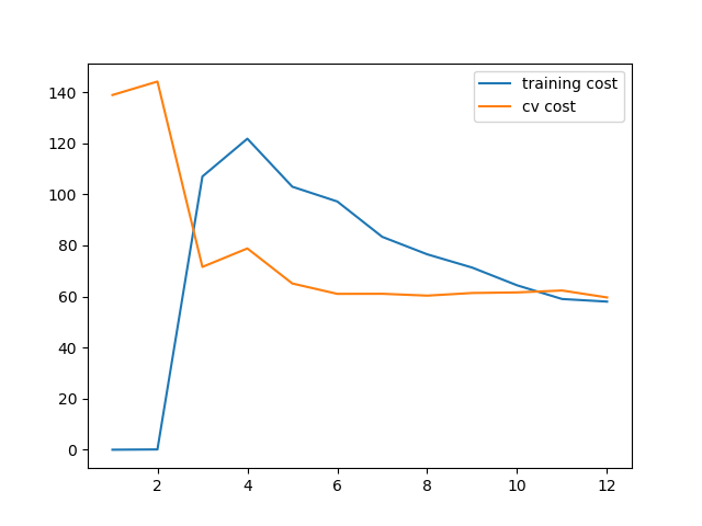
plot_learning_curve(X_poly, y, Xval_poly, yval, l=1)
plt.show()
plot_learning_curve(X_poly, y, Xval_poly, yval, l=100)
plt.show()

当λ取0时，也就是没有正则项时，可以看到训练的代价太低了，不真实. 这是过拟合了

当训练代价增加了些，不再是0了。稍减轻了过拟合

当λ取100时，正则化过多，变成了欠拟合。

最优λ

# 找到最佳拟合
l_candidate = [0, 0.001, 0.003, 0.01, 0.03, 0.1, 0.3, 1, 3, 10]
training_cost, cv_cost = [], []
for l in l_candidate:
    theta = np.ones(X_poly.shape[1])
    theta = linear_regression_np(theta, X_poly, y, l)[0]

    tc = cost(theta, X_poly, y)
    cv = cost(theta, Xval_poly, yval)
    training_cost.append(tc)
    cv_cost.append(cv)

plt.plot(l_candidate, training_cost, label='training')
plt.plot(l_candidate, cv_cost, label='cross validation')
plt.legend(loc=2)
plt.xlabel('lambda')
plt.ylabel('cost')
plt.show()


# best cv I got from all those candidates
l_candidate[np.argmin(cv_cost)]

# use test data to compute the cost
for l in l_candidate:
    theta = np.ones(X_poly.shape[1])
    theta = linear_regression_np(theta, X_poly, y, l)[0]
    print('test cost(l={}) = {}'.format(l, cost(theta, Xtest_poly, ytest)))

test cost(l=0) = 9.799399498688892
test cost(l=0.001) = 11.054987989655938
test cost(l=0.003) = 11.249198861537238
test cost(l=0.01) = 10.879605199670008
test cost(l=0.03) = 10.022734920552129
test cost(l=0.1) = 8.632060998872074
test cost(l=0.3) = 7.336602384055533
test cost(l=1) = 7.46630349664086
test cost(l=3) = 11.643928200535115
test cost(l=10) = 27.715080216719304

调参后， lambda = 0.3 是最优选择，这个时候测试代价最小