ex4-NN back propagation
AndrewNg 机器学习习题ex4-NN back propagation
需要的头:
import matplotlib.pyplot as plt
import numpy as np
import scipy.io as sio
import matplotlib
import scipy.optimize as opt
from sklearn.metrics import classification_report # 这个包是评价报告
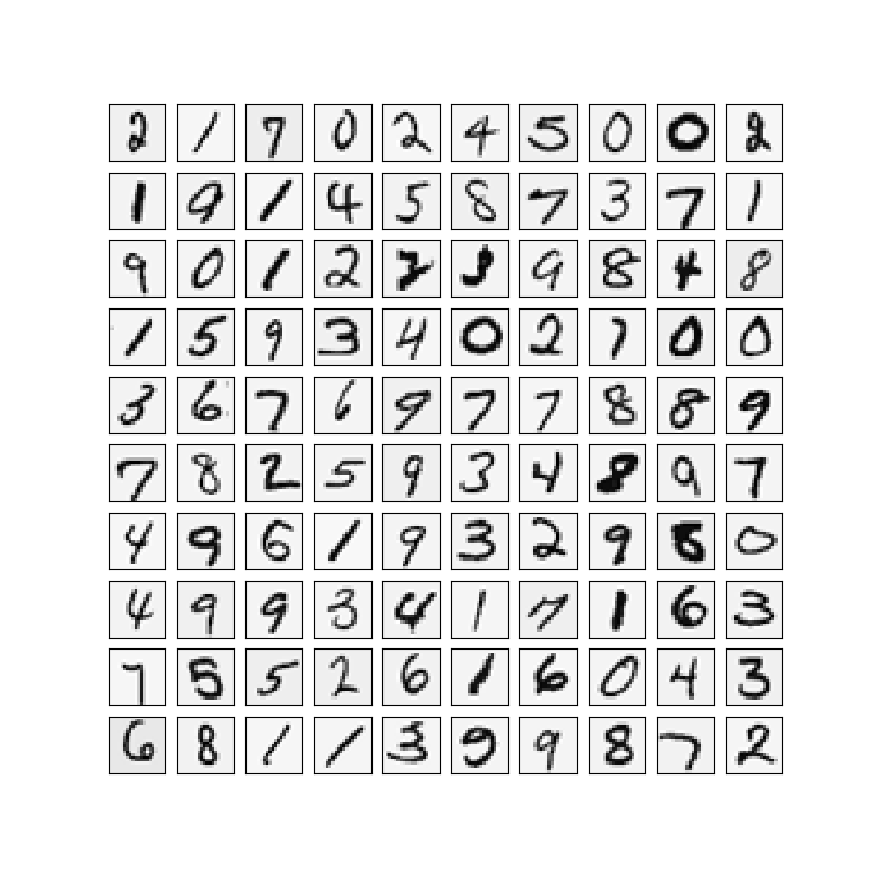
Visualizing the data
载入数据:
def load_data(path, transpose=True):
    data = sio.loadmat(path)
    y = data.get('y')
    y = y.reshape(y.shape[0])
    X = data.get('X')
    if transpose:
        X = np.array([im.reshape((20, 20)).T for im in X])
        X = np.array([im.reshape(400) for im in X])
    return X, y


X, y = load_data('./data/ex4data1.mat')


def plot_100_image(X):
    size = int(np.sqrt(X.shape[1]))
    sample_idx = np.random.choice(np.array(X.shape[0]), 100)
    sample_images = X[sample_idx, :]

    fig, ax_array = plt.subplots(nrows=10, ncols=10, sharey=True, sharex=True, figsize=(8, 8))

    for r in range(10):
        for c in range(10):
            ax_array[r, c].matshow(sample_images[10 * r + c].reshape((size, size)), cmap=matplotlib.cm.binary)
            plt.xticks(np.array([]))
            plt.yticks(np.array([]))
    plt.show()
plot_100_image(X)
准备数据
特征集合X添加一列全为1的偏差向量,把目标向量y进行OneHot编码。
X_raw, y_raw = load_data('./data/ex4data1.mat', transpose=False) # 这里转置
X = np.insert(X_raw, 0, np.ones(X_raw.shape[0]), axis=1) # 增加全为1的一列
print(y.shape) # (5000,)
y = np.array([y_raw]).T
from sklearn.preprocessing import OneHotEncoder
encoder = OneHotEncoder(sparse=False)
y_onehot = encoder.fit_transform(y)
print(y_onehot.shape) # (5000, 10)
读取权重
先读取出ex4weights.mat中的theta1和theta2,把theta展开后进行扁平化处理。
def load_weight(path):
    data = sio.loadmat(path)
    return data['Theta1'], data['Theta2']


t1, t2 = load_weight('./data/ex4weights.mat')
print(t1.shape, t2.shape) # (25, 401) (10, 26)


def serialize(a, b):
    # np.ravel() 降维
    # np.concatenate() 拼接
    return np.concatenate((np.ravel(a), np.ravel(b)))


def deserialize(seq):
    # 解开为两个theta
    return seq[:25 * 401].reshape(25, 401), seq[25 * 401:].reshape(10, 26)


theta = serialize(t1, t2)
print(theta.shape)  # (25 * 401) + (10 * 26) = 10285
前向传播 feed forward
(400 + 1) -> (25 + 1) -> (1)

def sigmoid(z):
    return 1 / (1 + np.exp(-z))


def feed_forward(theta, X):
    t1, t2 = deserialize(theta)
    m = X.shape[0]

    a1 = X # 5000 * 401
    z2 = a1 @ t1.T
    a2 = np.insert(sigmoid(z2), 0, np.ones(m), axis=1)  # 5000*26 第一列加一列一
    z3 = a2 @ t2.T  # 5000 * 100
    h = sigmoid(z3)  # 5000 * 10 这是 h_theta(X)

    return a1, z2, a2, z3, h  # 把每一层的计算都返回

#_, _, _, _, h = feed_forward(theta, X)

#print(h.shape) # (5000, 10)
代价函数与正则化


def cost(theta, X, y):
    m = X.shape[0]
    _, _, _, _, h = feed_forward(theta, X)
    pair_computation = -np.multiply(y, np.log(h)) - np.multiply((1 - y), np.log(1 - h))
    return pair_computation.sum() / m


cost_res = cost(theta, X, y)
print("cost:",cost_res)


def regularized_cost(theta, X, y, l=1):
    t1, t2 = deserialize(theta)  # t1: (25,401) t2: (10,26)
    m = X.shape[0]

    reg_t1 = np.power(t1[:, 1:], 2).sum()
    reg_t2 = np.power(t2[:, 1:], 2).sum()
    reg = (1 / (2 * m)) * (reg_t1 + reg_t2)

    return cost(theta, X, y) + reg


regularized_cost_res = regularized_cost(theta, X, y)
print("reg cost:",regularized_cost_res)
反向传播
def sigmoid_gradient(z):
    return np.multiply(sigmoid(z), 1 - sigmoid(z))


print(sigmoid_gradient(0))  #0.25


def gradient(theta, X, y):
    t1, t2 = deserialize(theta)
    m = X.shape[0]
    deltal = np.zeros(t1.shape)
    delta2 = np.zeros(t2.shape)

    a1, z2, a2, z3, h = feed_forward(theta, X)

    for i in range(m):
        a1i = a1[i, :]
        z2i = z2[i, :]
        a2i = a2[i, :]

        hi = h[i, :]
        yi = y[i, :]

        d3i = hi - yi

        z2i = np.insert(z2i, 0, np.ones(1))
        d2i = np.multiply(t2.T @ d3i, sigmoid_gradient(z2i))

        delta2 += np.matrix(d3i).T @ np.matrix(a2i)
        deltal += np.matrix(d2i[1:]).T @ np.matrix(a1i)


    delta1 = deltal / m
    delta2 = delta2 / m

    return serialize(delta1, delta2)


d1, d2 = deserialize(gradient(theta, X, y))
print(d1.shape, d2.shape) # (25, 401) (10, 26)
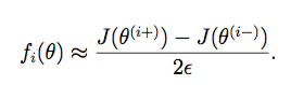
梯度校验
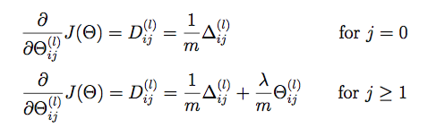
梯度正则化:
def regularized_gradient(theta, X, y, l=1):
    """don't regularize theta of bias terms"""
    m = X.shape[0]
    delta1, delta2 = deserialize(gradient(theta, X, y))
    t1, t2 = deserialize(theta)

    t1[:, 0] = 0
    reg_term_d1 = (l / m) * t1
    delta1 = delta1 + reg_term_d1

    t2[:, 0] = 0
    reg_term_d2 = (l / m) * t2
    delta2 = delta2 + reg_term_d2

    return serialize(delta1, delta2)

def expand_array(arr):
    """replicate array into matrix
    [1, 2, 3]

    [[1, 2, 3],
     [1, 2, 3],
     [1, 2, 3]]
    """
    # turn matrix back to ndarray
    return np.array(np.matrix(np.ones(arr.shape[0])).T @ np.matrix(arr))

def gradient_checking(theta, X, y, epsilon, regularized=False):
    def a_numeric_grad(plus, minus, regularized=False):
        """calculate a partial gradient with respect to 1 theta"""
        if regularized:
            return (regularized_cost(plus, X, y) - regularized_cost(minus, X, y)) / (epsilon * 2)
        else:
            return (cost(plus, X, y) - cost(minus, X, y)) / (epsilon * 2)

    theta_matrix = expand_array(theta)  # expand to (10285, 10285)
    epsilon_matrix = np.identity(len(theta)) * epsilon

    plus_matrix = theta_matrix + epsilon_matrix
    minus_matrix = theta_matrix - epsilon_matrix

    # calculate numerical gradient with respect to all theta
    numeric_grad = np.array([a_numeric_grad(plus_matrix[i], minus_matrix[i], regularized)
                                    for i in range(len(theta))])

    # analytical grad will depend on if you want it to be regularized or not
    analytic_grad = regularized_gradient(theta, X, y) if regularized else gradient(theta, X, y)

    # If you have a correct implementation, and assuming you used EPSILON = 0.0001
    # the diff below should be less than 1e-9
    # this is how original matlab code do gradient checking
    diff = np.linalg.norm(numeric_grad - analytic_grad) / np.linalg.norm(numeric_grad + analytic_grad)

    print('If your backpropagation implementation is correct,\nthe relative difference will be smaller than 10e-9 (assume epsilon=0.0001).\nRelative Difference: {}\n'.format(diff))


# gradient_checking(theta, X, y, epsilon= 0.0001)#这个运行很慢,谨慎运行
If your backpropagation implementation is correct,
the relative difference will be smaller than 10e-9 (assume epsilon=0.0001).
Relative Difference: 2.1466000818218673e-09
准备训练模型
def random_init(size):
    return np.random.uniform(-0.12, 0.12, size)

def nn_training(X, y):
    init_theta = random_init(10285) # 25 * 401 + 10 * 26

    res = opt.minimize(fun=regularized_cost,
                       x0=init_theta,
                       args=(X ,y, 1),
                       method='TNC',
                       jac=regularized_gradient,
                       options={'maxiter': 400})
    return res

res = nn_training(X, y) # 慢
print(res)
Out put:
     fun: 0.32211992072588747
     jac: array([ 2.15004329e-04,  3.88985627e-08, -3.33174201e-08, ...,
        3.15328424e-05,  2.82831419e-05, -1.68082404e-05])
 message: 'Max. number of function evaluations reached'
    nfev: 400
     nit: 26
  status: 3
 success: False
       x: array([ 0.00000000e+00,  1.94492814e-04, -1.66587101e-04, ...,
       -7.15493763e-01, -1.36561388e+00, -2.90127262e+00])
显示准确率
_, y_answer = load_data('./data/ex4data1.mat')

final_theta = res.x

def show_accuracy(theta, X, y):
    _, _, _, _, h = feed_forward(theta, X)

    y_pred = np.argmax(h, axis=1) + 1

    print(classification_report(y, y_pred))

show_accuracy(final_theta, X, y_answer)
Out Put:
             precision    recall  f1-score   support

          1       1.00      0.79      0.88       500
          2       0.73      1.00      0.85       500
          3       0.82      0.99      0.89       500
          4       1.00      0.89      0.94       500
          5       1.00      0.86      0.92       500
          6       0.94      0.99      0.97       500
          7       0.99      0.81      0.89       500
          8       0.94      0.95      0.95       500
          9       0.96      0.95      0.95       500
         10       0.96      0.98      0.97       500

avg / total       0.93      0.92      0.92      5000
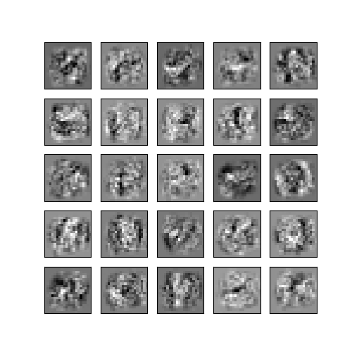
显示隐藏层
def plot_hidden_layer(theta):
    """
    theta: (10285, )
    """
    final_theta1, _ = deserialize(theta)
    hidden_layer = final_theta1[:, 1:]  # ger rid of bias term theta

    fig, ax_array = plt.subplots(nrows=5, ncols=5, sharey=True, sharex=True, figsize=(5, 5))

    for r in range(5):
        for c in range(5):
            ax_array[r, c].matshow(hidden_layer[5 * r + c].reshape((20, 20)),
                                   cmap=matplotlib.cm.binary)
            plt.xticks(np.array([]))
            plt.yticks(np.array([]))

plot_hidden_layer(final_theta)
plt.show()