ex3-neural network
AndrewNg 机器学习习题ex3-neural network
ex3data1.mat是一个matlab文件,储存了5000个图像的数据,每个图像是一个20像素×20像素的灰度图,展开后为一个400维的向量,每一个向量都储存为矩阵X的行,所以X的维度是(5000,400)
y的每一行代表X所对应的手写数字,y的维度是(5000,1)
需要的头:
import matplotlib.pyplot as plt
import numpy as np
import scipy.io as sio
import matplotlib
import scipy.optimize as opt
from sklearn.metrics import classification_report # 这个包是评价报告
Visualizing the data
载入数据:
def load_data(path, transpose=True):
    data = sio.loadmat(path)
    y = data.get('y')
    y = y.reshape(y.shape[0])
    X = data.get('X')
    if transpose:
        X = np.array([im.reshape((20, 20)).T for im in X])
        X = np.array([im.reshape(400) for im in X])
    return X, y

X, y = load_data('./data/ex3data1.mat')
画一个图
def plot_an_image(image):
    fig, ax = plt.subplots(figsize=(1, 1))
    ax.matshow(image.reshape((20, 20)), cmap=matplotlib.cm.binary)
    plt.xticks(np.array([]))
    plt.yticks(np.array([]))
    plt.show()

pick_one = np.random.randint(0, 5000)
plot_an_image(X[pick_one, :])
print('this should be {}'.format(y[pick_one]))

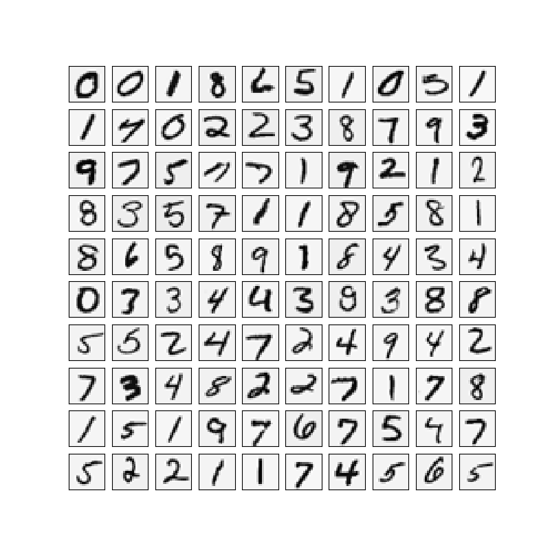
画一百个图
def plot_100_image(X):
    size = int(np.sqrt(X.shape[1]))
    sample_idx = np.random.choice(np.array(X.shape[0]), 100)
    sample_images = X[sample_idx, :]

    fig, ax_array = plt.subplots(nrows=10, ncols=10, sharey=True, sharex=True, figsize=(8, 8))

    for r in range(10):
        for c in range(10):
            ax_array[r, c].matshow(sample_images[10 * r + c].reshape((size, size)), cmap=matplotlib.cm.binary)
            plt.xticks(np.array([]))
            plt.yticks(np.array([]))
    plt.show()

plot_100_image(X)
准备数据
加载好ex3data1.mat文件后我们需要处理一下,首先X是一个(5000,400)的矩阵,我们在第一列加上一列全为1的矩阵为偏差量,y是一个(5000,)的矩阵,需要注意的是,为了兼容Oxtave和matlab,y中0的被标记为了10。我们把y分成10类整理y数据为(10,5000)的一个矩阵。
扩展 5000*1 到 5000*10
     比如 y=10 -> [0, 0, 0, 0, 0, 0, 0, 0, 0, 1]: ndarray
     比如 y=1 -> [0, 1, 0, 0, 0, 0, 0, 0, 0, 0]: ndarray
raw_X, raw_y = load_data('./data/ex3data1.mat')
X = np.insert(raw_X, 0, values=np.ones(raw_X.shape[0]), axis = 1) # 插入了第一列 全为1
y_matrix = []
for k in range(1, 11):
    y_matrix.append((raw_y == k).astype(int))
y_matrix = [y_matrix[-1]] + y_matrix[:-1]
y = np.array(y_matrix)
训练一维模型
处理好数据后接着写,激活函数和代价函数,代价函数的偏导数就是梯度函数,我们期望这个函数最小。给梯度函数和代价函数加入正则项。
def sigmoid(z):
    return 1 / (1 + np.exp(-z))

def cost(theta, X, y):
    return np.mean(-y * np.log(sigmoid(X @ theta)) - (1 - y) * np.log(1 - sigmoid(X @ theta)))

# 梯度就是jθ的在θ偏导
def gradient(theta, X, y):
    # @ 对应元素相乘求和
    return (1 / len(X)) * X.T @ (sigmoid(X @ theta) - y)

def regularized_cost(theta, X, y, l=1):
    theta_j1_to_n = theta[1:]
    regularized_term = (1 / (2 * len(X))) * np.power(theta_j1_to_n, 2).sum()

    return cost(theta, X, y) + regularized_term

def regularized_gradient(theta, X, y, l=1):
    theta_j1_to_n = theta[1:]
    regularized_theta = (l / len(X)) * theta_j1_to_n
    regularized_term = np.concatenate([np.array([0]), regularized_theta]) # 在theta矩阵前接一个[0]
    return gradient(theta, X, y) + regularized_term
运用minimize()函数开始迭代,计算出theta,然后验证theta的准确性。
def logistic_regression(X, y, l=1):
    theta = np.zeros(X.shape[1])
    res = opt.minimize(fun=regularized_cost, x0=theta, args=(X, y, l), method='TNC', jac=regularized_gradient, options={'disp': True})
    final_theta = res.x
    return final_theta

def predict(x, theta):
    prob = sigmoid(x @ theta)
    return (prob >= 0.5).astype(int)

t0 = logistic_regression(X, y[0])
y_pred = predict(X, t0)
print('Accuracy={}'.format(np.mean(y[0] == y_pred)))
最终求得结果为 Accuracy=0.9974
训练K维模型
k_theta = np.array([logistic_regression(X, y[k]) for k in range(10)])
print(k_theta.shape) # (10, 401)

prob_matrix = sigmoid(X @ k_theta.T)
np.set_printoptions(suppress=True) # 科学计数法表示
print(prob_matrix.shape) # (5000, 10)

y_pred = np.argmax(prob_matrix, axis=1)
print(y_pred.shape) # (5000,)

y_answer = raw_y.copy()
y_answer[y_answer==10] = 0

print(classification_report(y_answer, y_pred))
             precision    recall  f1-score   support

          0       0.97      0.99      0.98       500
          1       0.95      0.99      0.97       500
          2       0.95      0.92      0.93       500
          3       0.95      0.91      0.93       500
          4       0.95      0.95      0.95       500
          5       0.92      0.92      0.92       500
          6       0.97      0.98      0.97       500
          7       0.95      0.95      0.95       500
          8       0.93      0.92      0.92       500
          9       0.92      0.92      0.92       500

avg / total       0.94      0.94      0.94      5000
如ex3.pdf中所说,我们成功的分类出94%的例子。
Feedforward Propagation and Prediction
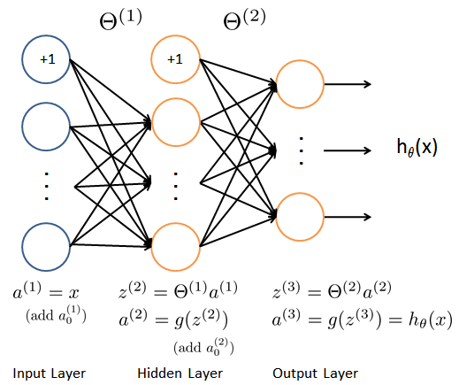
我们的神经网路如上图所示,它有3层构成(一个输入层,一个隐藏层a,一个输出层。)已经提供了一组训练参数(Θ1,Θ2)储存在ex3weights.mat中
% Load saved matrices from file
load('ex3weights.mat');
% The matrices Theta1 and Theta2 will now be in your Octave
% environment
% Theta1 has size 25 x 401
% Theta2 has size 10 x 26
def load_weight(path):
    data = sio.loadmat(path)
    return data['Theta1'], data['Theta2']

theta1, theta2 = load_weight('./data/ex3weights.mat')

X, y = load_data('./data/ex3data1.mat',transpose=False)

X = np.insert(X, 0, values=np.ones(X.shape[0]), axis=1)  # intercept

a1 = X

z2 = a1 @ theta1.T # (5000, 401) @ (25,401).T = (5000, 25)
print(z2.shape)

z2 = np.insert(z2, 0, values=np.ones(z2.shape[0]), axis=1)

a2 = sigmoid(z2)

z3 = a2 @ theta2.T

a3 = sigmoid(z3)

y_pred = np.argmax(a3, axis=1) + 1  # numpy is 0 base index, +1 for matlab convention,返回沿轴axis最大值的索引,axis=1代表行

print(classification_report(y, y_pred))
             precision    recall  f1-score   support

          1       0.97      0.98      0.97       500
          2       0.98      0.97      0.97       500
          3       0.98      0.96      0.97       500
          4       0.97      0.97      0.97       500
          5       0.98      0.98      0.98       500
          6       0.97      0.99      0.98       500
          7       0.98      0.97      0.97       500
          8       0.98      0.98      0.98       500
          9       0.97      0.96      0.96       500
         10       0.98      0.99      0.99       500

avg / total       0.98      0.98      0.98      5000